← Harley Turan•April 2022

Visualizing Complex Numbers Using GLSL

Intrigued by this series of tweets by Keenan Crane (and this exploration by Varun Vachhar), I spent a recent Sunday morning dusting off high school memories of complex numbers in order to write some pretty shaders.

Keenan’s tweet showed a few formulas visualized in 2D space, and I was immediately faced with a couple of questions:

What does any of this mean?
How do I make art using it?

Hopefully this post helps break down what’s going on here (or at least to the best of my understanding), and how we can use what we learn to play with and visualize complex numbers.

GLSL, or the OpenGL Shading Language, is a graphics programming language that can be used to program visual effects. Shaders are both incredibly versatile and also conceptually simple — you write a set of instructions, and those instructions are run for every pixel on the screen. The result of those instructions tells the pixel what color it should display as.

Whilst conceptually simple, shaders can be really complex to work with. Instead of thinking “I want to make the 62nd pixel across and the 38th pixel down be red” (as seen in my seminal work Red Pixel, 2019), we need to think in mathematical terms about the shape of functions in 2D space. Lots of trigonometry and obscure functions to make shapes. The Book of Shaders is a lovely introduction.

The visuals we'll be creating today are all really just vizualising math — drawn on a flat screen and given colors. Zach Lieberman (of the School for Poetic Computation and MIT Media Lab) put this well recently:

So! Math…

To start with, let’s talk about complex numbers, because they’re fun and weird.

At a high level, Complex numbers are numbers that are split into two parts — real and imaginary. They are represented in the form $a + bi$ , where $a$ and $b$ are real numbers, and $i$ is the imaginary unit (representing $\sqrt{-1}$ , an impossible number).

Just like me, GLSL doesn't really understand complex numbers, so our job here is to represent them in a way that we're both familiar with.

Luckily, as $a$ and $b$ are real numbers, we can do real number things with them! They can be represented in GLSL as regular floating point values (float), and stored in a floating-point vec2 vector (just a set of two floats). By representing our complex number like this, we can perform complex arithmetic on it and have GLSL able to follow along.

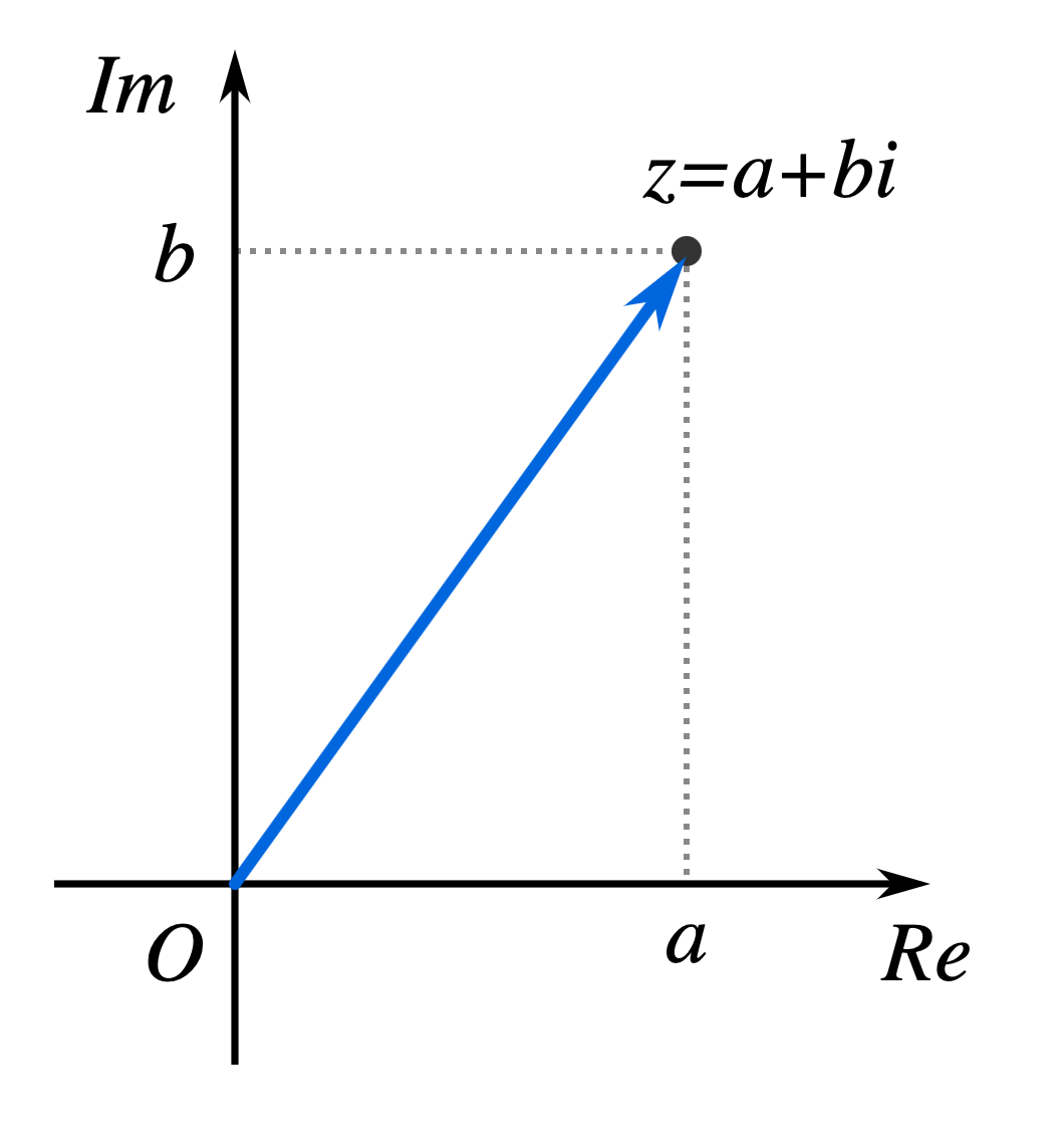
Also, as with anything we can represent with two values, we can then visualize these values on a 2D surface (known as the "complex plane" when dealing with complex numbers). On the complex plane, the horizontal x-axis represents $a$ , our real component ( $\operatorname{Re}$ , the real axis), and the vertical y-axis represents $b$ , our imaginary component ( $\operatorname{Im}$ , the imaginary axis).

Welcome to the first “well, actually…” aside.

For our purposes, we're more interested in plotting these complex numbers onto the complex plane in a polar form, rather than the cartesian form we just described. To plot polar coordinates around our origin, we need to represent our complex number as a modulus and an argument.

The length of the line from the origin to point $z$ is known as the modulus ( $|z|$ or $r$ ), and we can calculate it using Pythagorus’ theorem, where $|z| = \sqrt{a^2 + b^2}$ . The angle between the line and the real axis is known as the argument of the complex number ( $\varphi$ ). This can be calculated using trigonometry, where $\varphi = atan2(b, a)$ .

This Youtube series covers a lot of the specifics with far, far more detail, intelligence, and engagement than I ever could. Wikipedia also has some wonderful visualizations of $\varphi = atan2(b, a)$ plotted in 3D space, and great descriptions of log-polar coordinates which really helped me understand where the "lines" or "edges" in our produced gradients are coming from.

Now that I've written some $\LaTeX$ and it’s given me the false confidence that I know what I’m talking about, let’s break down the formula in Keenan’s first tweet above:

\operatorname{Im}(\log(\frac{z-p}{z-q}))

Here’s what we're working with —

$z$ is our complex number (we'll be using it as our $x$ and $y$ coordinates for each point on the plane, or our uv.xy if you're already familiar with shader programming)
$p$ and $q$ are both arbitrary points on the plane between which we'll draw a line
$\log$ is the complex logarithm
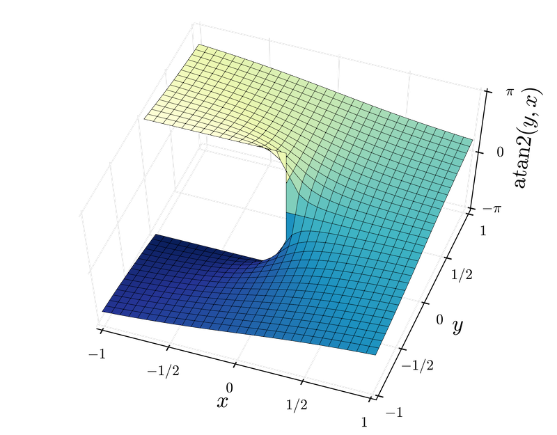
$\operatorname{Im}$ is the imaginary part of our complex number (you'll also often see $\operatorname{Re}$ for the real part).

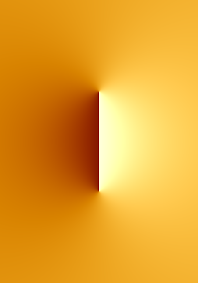
What we're doing here is effectively plotting the complex logarithm between two points on the complex plane. It‘s easy for me to write that as if I know what it means or what we’ll see when we do the math, but I’m confident it’ll look good regardless. Let‘s press on!

Right now, we have a complex plane (our GLSL canvas), we have some complex numbers we can put on the plane (our pixels and points), and we have the ability to perform arithmetic on them (the instructions we’ll write in GLSL). Let’s write some shader code!

glsl

vec2 uv = (gl_FragCoord.xy - 0.5 * u_resolution.xy) / min(u_resolution.y, u_resolution.x);
vec2 z = uv;

Here, gl_FragCoord is the xy coordinate of the fragment (the pixel we're working on), and u_resolution is the resolution of our canvas we'll be rendering to. What we're doing here is setting our bounds — rather than working with values matching the resolution (say, 500, 500 for a 500px square canvas), we're taking our pixel coordinate and mapping it to the range -0.5, 0.5 (with some aspect ratio correction thrown in using min).

As mentioned before, we'll be using $z$ in math terms as our uv in shader terms, meaning that for our purposes, each pixel on the screen is now represented as a complex number.

Let’s also define our static points $p$ and $q$ between which we'll draw a line:

glsl

// Lower-left point
vec2 p = vec2(-0.25, -0.25);

// Upper-right point
vec2 q = vec2(0.25, 0.25);

And with all the parameters now defined, we can convert our formula $\operatorname{Im}(\log(\frac{z-p}{z-q}))$ to GLSL:

glsl

// Divide z-p by z-q using complex division
vec2 division = cx_div((z - p), (z - q));

// Calculate the log of our division
vec2 log_p_over_q = cx_log(division);

// Extract the imaginary number
float imaginary = log_p_over_q.y;

And there we have it — a float value for our shader to paint to the screen.

You might notice that we're not doing (z - p) / (z - q) here.

When dealing with complex and vector arithmetic, there’s a little translation needed to work with GLSL. GLSL performs component-wise vector arithmetic, which is different from what we traditionally see in linear arithmetic.

In GLSL, multiplying a vec2 of $(a, b)$ by a vec2 of $(c, d)$ results in a vec2 of $(ac, bd)$ , but when we multiply two imaginary numbers together, we get $(ac - bd) + (ad + bc)i$ .

To help with this, we can define some functions for complex arithmetic —

glsl

// From https://github.com/julesb/glsl-util

#define PI 3.14159265

#define cx_mul(a, b) vec2(a.x*b.x - a.y*b.y, a.x*b.y + a.y*b.x)
#define cx_div(a, b) vec2(((a.x*b.x + a.y*b.y)/(b.x*b.x + b.y*b.y)),((a.y*b.x - a.x*b.y)/(b.x*b.x + b.y*b.y)))
#define cx_sin(a) vec2(sin(a.x) * cosh(a.y), cos(a.x) * sinh(a.y))
#define cx_cos(a) vec2(cos(a.x) * cosh(a.y), -sin(a.x) * sinh(a.y))

vec2 as_polar(vec2 z) {
  return vec2(
    length(z),
    atan(z.y, z.x)
  );
}

vec2 cx_tan(vec2 a) {return cx_div(cx_sin(a), cx_cos(a)); }
vec2 cx_log(vec2 a) {
    vec2 polar = as_polar(a);
    float rpart = polar.x;
    float ipart = polar.y;
    if (ipart > PI) ipart=ipart-(2.0*PI);
    return vec2(log(rpart),ipart);
}
vec2 cx_pow(vec2 v, float p) {
  vec2 z = as_polar(v);
  return pow(z.x, p) * vec2(cos(z.y * p), sin(z.y * p));
}

In our case here, the imaginary part of our complex logarithm is really just $\varphi$ , which is atan(z.y, z.x) (the .y returned from as_polar. The shader we‘re writing here can be simplified, but I find it helps to map one-to-one with the formula we’re trying to visualize.

Our imaginary value gives us everything we need, but it‘s just a float. Shaders output four numbers per pixel (red, green, blue, and alpha — RGBA), and we just have the one. To make things a little more visually-interesting, we can use Inigo Quilez’s procedural palette function to add some color to our current grayscale value:

glsl

// From https://iquilezles.org/www/articles/palettes/palettes.htm

vec3 palette( in float t, in vec3 a, in vec3 b, in vec3 c, in vec3 d )
{
    return a + b*cos(2. * PI *(c*t+d) );
}

This function takes in a float value — which for us is will be the imaginary part of our logarithm — along with four vec3s that can be altered endlessly to produce beautiful output.

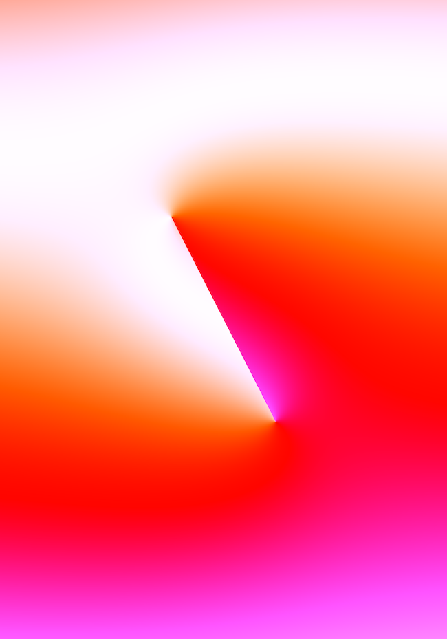
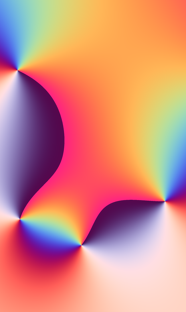
With all of these pieces combined (and some over-complicated tone-mapping using our palette function) we get the following:

glsl

#version 300 es
precision mediump float;

out vec4 fragColor;

uniform vec2 u_resolution;
uniform float u_time;

#define PI 3.141592653589793

#define cx_div(a, b) vec2(((a.x*b.x+a.y*b.y)/(b.x*b.x+b.y*b.y)),((a.y*b.x-a.x*b.y)/(b.x*b.x+b.y*b.y)))

vec2 as_polar(vec2 z) {
  return vec2(
    length(z),
    atan(z.y, z.x)
  );
}

vec2 cx_log(vec2 a) {
    vec2 polar = as_polar(a);
    float rpart = polar.x;
    float ipart = polar.y;
    if (ipart > PI) ipart=ipart-(2.0*PI);
    return vec2(log(rpart),ipart);
}

vec3 palette( in float t, in vec3 a, in vec3 b, in vec3 c, in vec3 d ) {
    return a + b*cos( 0.38*2.*PI*(c*t+d) );
}

void main() {
  vec2 uv = (gl_FragCoord.xy - 0.5 * u_resolution.xy) / min(u_resolution.y, u_resolution.x);
  vec2 z = uv;
  
  float angle = sin(u_time/5.) * 2. * PI;
  float length = .2;
  
  // Spin our points in a circle of radius length
  float c = cos(angle);
  float s = sin(angle);
  vec2 p = vec2( s*length, c*length);
  vec2 q = vec2( s*-length, c*-length );
  
  // Divide z-p by z-q using complex division
  vec2 division = cx_div((z - p), (z - q));
  
  // Calculate the log of our division
  vec2 log_p_over_q = cx_log(division);

  // Extract the imaginary number
  float imaginary = log_p_over_q.y / PI;

  vec3 col = palette( imaginary, vec3(0.50,.52,0.53), vec3(.46,.32,.35), vec3(.82,.84,.65), vec3(0.53,0.23,0.22));

  fragColor = vec4(col, 1.0);
}

As with any shader, by jamming a bunch of random numbers into the many float variables we have here (and by making some tweaks to how our values are rendered across .xy screen space), we can get output like the following —

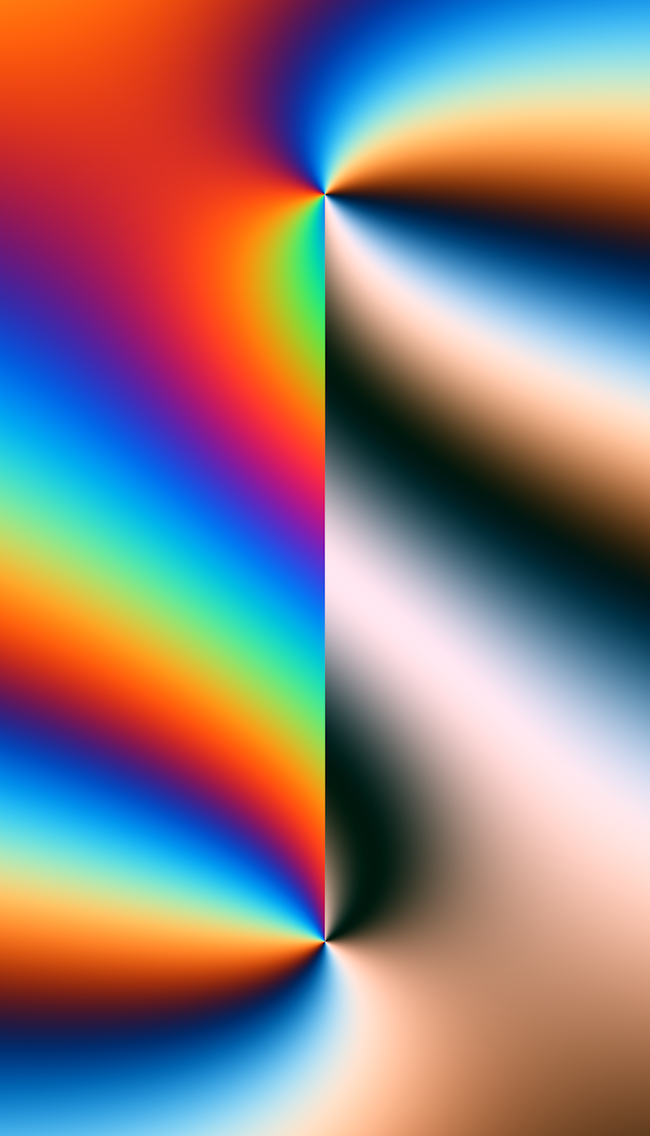
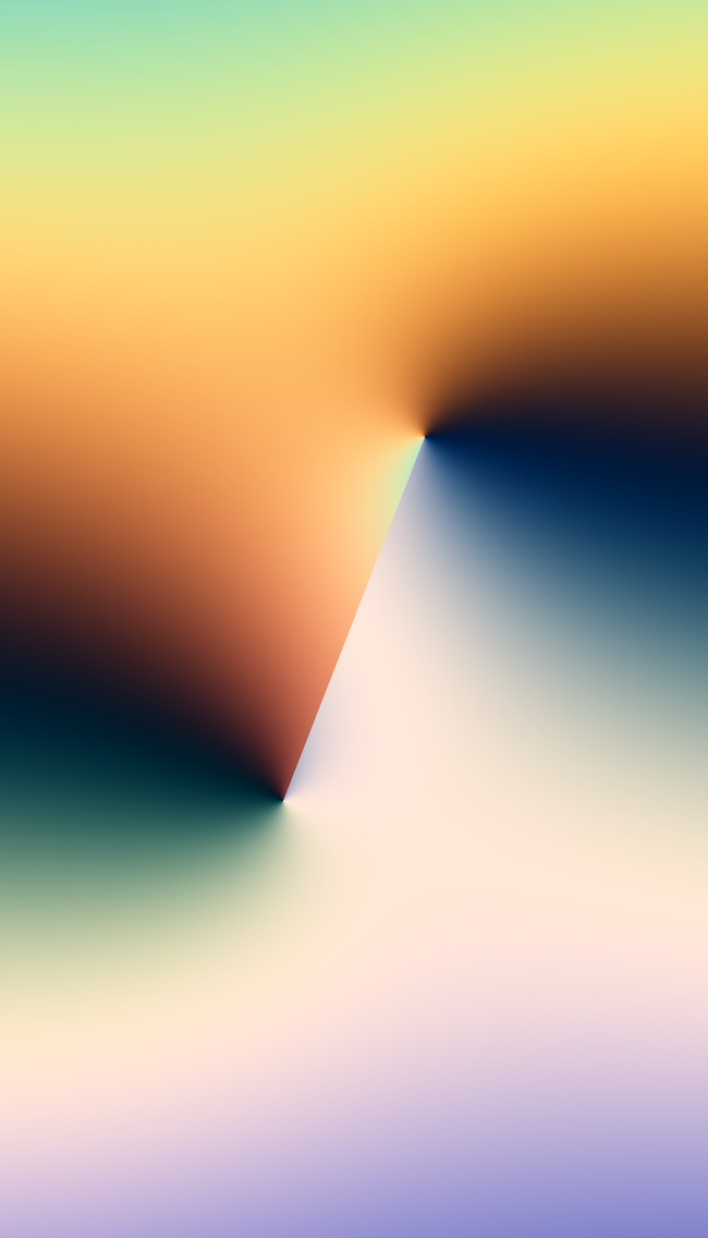
Beautiful! Who would imagine.

If you’ve got time and patience, I’ve got a little more math for you.

Keenan‘s original tweet actually showed a slightly more advanced representation of complex numbers, showing meromorphic functions (functions where certain points shoot off up to infinity) —

When we take a look at this function:

\operatorname{Im}(\log(\frac{\sum_{k=0}^{m} a_{k}z^{k}}{\sum_{k=0}^{n} b_{k}z^{k}}))

a_{0},\dots,a_{m},b_{0},\dots,b_{n}\in\mathbb{C}

We recognize some old friends — $\log$ , $\operatorname{Im}$ , $z$ — but also some new faces:

$a$ and $b$ are a set of arbitrary points (complex numbers) we'll be using to draw with.
$m$ and $n$ are just the number of points we'll be showing here, the total counts for $a$ and $b$
For those not familiar with sigma notation, $\sum_{k=0}^{m}$ just means "sum the following function $m$ times starting at $k$ "

That sigma statement in this case can be written out longhand as $a_{0}+a_{1}z+\dotsb+a_{m}z^{m}$ . In fact, if we set our limits $m$ and $n$ to $3$ , we get —

\operatorname{Im}(\log(\frac{a_{0}+a_{1}z+a_{2}z^{2}+a_{3}z^{3}}{b_{0}+b_{1}z+b_{2}z^{2}+b_{3}z^{3}}))

What this formula represents is the imaginary part of the complex logarithm of the ratio of two complex polynomials.

Okay, I know. That was a lot of math. I’m sorry.

With our $a$ and $b$ still representing x and y points on the complex plane, we can scatter some points around the complex plane and, like before, represent this formula in GLSL:

glsl

#version 300 es
precision mediump float;

out vec4 fragColor;

uniform vec2 u_resolution;
uniform float u_time;

#define PI 3.1415926535897932384626433832795

#define cx_mul(a, b) vec2(a.x*b.x - a.y*b.y, a.x*b.y + a.y*b.x)
#define cx_div(a, b) vec2(((a.x*b.x + a.y*b.y)/(b.x*b.x + b.y*b.y)),((a.y*b.x - a.x*b.y)/(b.x*b.x + b.y*b.y)))
#define cx_sin(a) vec2(sin(a.x) * cosh(a.y), cos(a.x) * sinh(a.y))
#define cx_cos(a) vec2(cos(a.x) * cosh(a.y), -sin(a.x) * sinh(a.y))

vec2 cx_tan(vec2 a) {return cx_div(cx_sin(a), cx_cos(a)); }
vec2 cx_log(vec2 a) {
    float rpart = sqrt((a.x*a.x)+(a.y*a.y));
    float ipart = atan(a.y,a.x);
    if (ipart > PI) ipart=ipart-(2.0*PI);
    return vec2(log(rpart),ipart);
}

vec2 as_polar(vec2 z) {
  return vec2(
    length(z),
    atan(z.y, z.x)
  );
}
vec2 cx_pow(vec2 v, float p) {
  vec2 z = as_polar(v);
  return pow(z.x, p) * vec2(cos(z.y * p), sin(z.y * p));
}

float im(vec2 z) {
  return ((atan(z.y, z.x) / PI) + 1.0) * 0.5;
}

vec3 pal( in float t, in vec3 a, in vec3 b, in vec3 c, in vec3 d )
{
    return a + b*cos(2.*PI*(c*t+d));
}

// Define our points
vec2 a0 = vec2(0.32, -0.45);
vec2 a1 = vec2(-0.49, -0.32);
vec2 a2 = vec2(-0.31, 0.38);
vec2 a3 = vec2(-0.12, 0.04);

vec2 b0 = vec2(-0.71, 0.53);
vec2 b1 = vec2(0.01, 0.23);
vec2 b2 = vec2(-0.24, 0.31);
vec2 b3 = vec2(-0.01, -0.42);

void main() {
    // Set up our imaginary plane
    vec2 uv = (gl_FragCoord.xy - 0.5 * u_resolution.xy) / min(u_resolution.y, u_resolution.x);
    vec2 z = uv * 2.;

    // Calculate the sum of our first polynomial
    vec2 polyA = a0
        + cx_mul(a1, z)
        + cx_mul(a2, cx_pow(z, 2.0))
        + cx_mul(a3, cx_pow(z, 3.0));

    // Calculate the sum of our second polynomial
    vec2 polyB = b0
        + cx_mul(b1, z)
        + cx_mul(b2, cx_pow(z, 2.))
        + cx_mul(b3, cx_pow(z, 3.));

    // Calculate the ratio of our complex polynomials
    vec2 result = cx_div(polyA, polyB);

    float imaginary = cx_log(result).y;
    float col = (imaginary / PI);

    fragColor = vec4(pal(col, vec3(.52,.45,.61),vec3(.40,.42,.31),vec3(.26,.30,.35),vec3(.15,.4,.4)),1.0);
}

By putting some wild values in, we can get some wild images out —

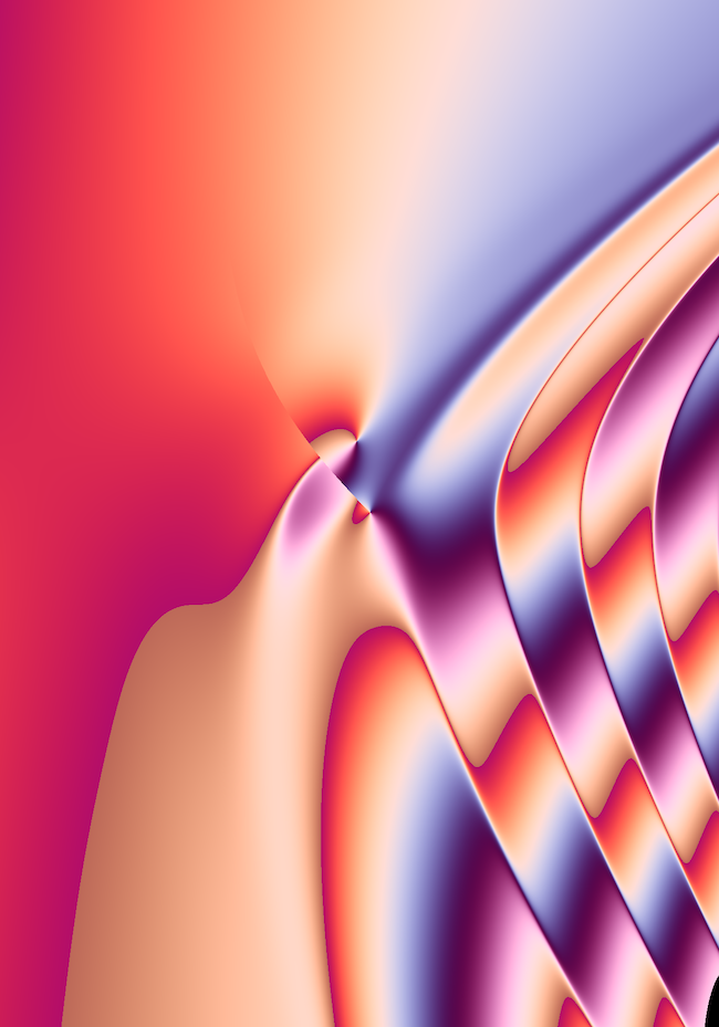
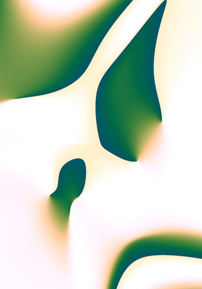
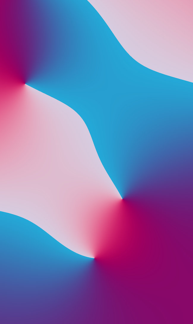
I don’t know about you, but I think Red Pixel, 2019 can go straight in the trash.

I find GLSL (and shaders in general) to be a fascinating medium. It is fundamentally a medium that can represent anything that can be pictured on a two-dimensional plane — 3D models, fractals, paintings, poetry, ink, photographs. If you can see it, you can create a shader to represent it. But more than this, if you can't see it, you can create a shader to represent it.

There are a lot of numbers out there.

Go see them.

❋

References

Fork Meromorphi mla 166 by mla

‌Fork Meromorphic Poly by akohdr

‌Complex Log x 3 by mla

‌The 5 ways to visualize complex functions by Mathemaniac

Domain Coloring Plot by Jim Fowler